시계열 예측 기법 (ARIMA)을 이용하거나, 최근에는 LSTM이나 AutoEncoder 등을 활용한 딥러닝 기반 방법론을 통해 시계열 데이터에서 이상탐지가 가능하다. 딥러닝 계열의 이상탐지가 성능이 우수하다고 일반적으로 알려 있으나, 1) 충분한 데이터 확보가 어렵고(매출이나 날씨 데이터는 기껏해야 하루 단위로 확보 가능하고, 그나마도 계절성을 고려하면 수십년을 모아야하는 경우도 있다), Supervised Learning은 정답 세트를 필요로 한다.
지수 평활법(Exponential Smoothing)은 ARIMA와 유사하게, Trend, Level, Seasonality를 활용하지만, 최근의 결과값에 더 무게를 준다거나 줄일 수 있다는 점이 다르다. 지수평활법은 단순히 Trend와 Level만 참조하는 SES(Single Exponential Smoothing)과 Seasonality까지 고려하는 Holt-Winters 모델이 있는데, 여기서는 후자를 간략하게 테스트 해 본다.
인도의 8년 데이터 중, 추세를 반영할 때 이상이 나타난 월(month)을 찾아내는 예제다. 아래 github의 데이터를 활용했고, 코드도 대부분 차용했으나 일부 간단하게 만들었다.
KrishnanSG/holt-winters
The repository provides an in-depth analysis and forecast of a time series dataset as an example and summarizes the mathematical concepts required to have a deeper understanding of Holt-Winter'...
github.com
# Imports for data visualization
import matplotlib.pyplot as plt
import pandas as pd
from matplotlib.dates import DateFormatter
from matplotlib import dates as mpld

temp_df = pd.read_csv('dataset/average_temp_india.csv')
temp_df['date'] = pd.to_datetime(temp_df['date'])
temp_df = temp_df.set_index('date')

# 앞의 70% 데이터만 학습에 사용
train_df = temp_df.iloc[:int(len(temp_df)*0.7)]
test_df = temp_df.iloc[int(len(temp_df)*0.7):]

plt.plot(temp_df['values'])
plt.gcf().autofmt_xdate()
plt.show()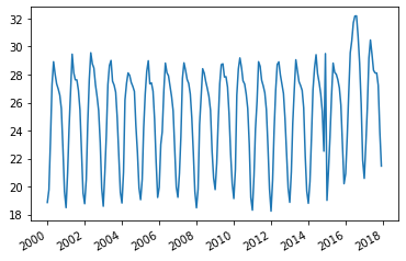
간단한 EDA만으로 2016년 이후 이상점들이 눈에 보이나, 일단 더 세분화 해보자
from statsmodels.tsa.seasonal import seasonal_decompose

seasonal_decompose(temp_df,model='additive',period=12).plot()
plt.show()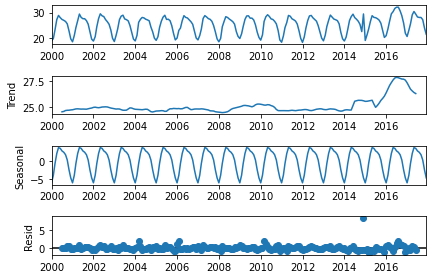
2016년에 에러도 커진 부분이 있고, 무엇보다 2015년 이후 Trend가 급상승하는 면이 있다. Seasonality는 유지되어 보인다. 이제 Holts-Winters 알고리즘으로 이상 포인트들을 찾아내 보자
from statsmodels.tsa.holtwinters import ExponentialSmoothing

# ES 모델을 만들어 학습하고 전체 데이터에 대해 예측한다.
# additive는 경향성이 일정함을 의미하고, 경향성 변동폭이 있을 때는 multiplicative를 사용
model = ExponentialSmoothing(
    train_df, trend='additive', seasonal='additive').fit()

prediction = model.predict(
    start=temp_df.index[0], end=temp_df.index[-1])

"""Brutlag Algorithm"""
PERIOD = 12        # The given time series has seasonal_period=12
GAMMA = 0.3684211  # the seasonility component
SF = 1.96          # brutlag scaling factor for the confidence bands.
UB = []            # upper bound or upper confidence band
LB = []            # lower bound or lower confidence band

# 실측치와 예측치를 비교하는 자료구조
difference_array = []
dt = []
difference_table = {"actual": temp_df, "predicted": prediction, "difference": difference_array, "UB": UB, "LB": LB}

# brutlag 알고리즘
# 12개월 이전의 실측/결측 차이에 0.63, 이번달 차이에 0.37 정도의 가중치를 주어 저장
for i in range(len(prediction)):
    diff = temp_df.iloc[i]-prediction.iloc[i]
    if i < PERIOD:
        dt.append(GAMMA*abs(diff))
    else:
        dt.append(GAMMA*abs(diff) + (1-GAMMA)*dt[i-PERIOD])

# 저장된 실측/결측 차이를 예측치의 95% 신뢰구간(1.96)으로 반영하여 Upper/Lower Band 계산
    difference_array.append(diff)
    UB.append(prediction[i]+SF*dt[i])
    LB.append(prediction[i]-SF*dt[i])

"""Classification of data points as either normal or anomaly"""
normal = []
normal_date = []
anomaly = []
anomaly_date = []

# 신뢰구간을 벗어나는지 판단하여 normal, anomaly 결정
for i in range(len(temp_df.index)):
    if ((UB[i] <= temp_df.iloc[i]).bool() or (LB[i] >= temp_df.iloc[i]).bool()) and i > PERIOD:
        anomaly_date.append(temp_df.index[i])
        anomaly.append(temp_df.iloc[i][0])
    else:
        normal_date.append(temp_df.index[i])
        normal.append(temp_df.iloc[i][0])

anomaly = pd.DataFrame({"date": anomaly_date, "value": anomaly})
anomaly.set_index('date', inplace=True)
normal = pd.DataFrame({"date": normal_date, "value": normal})
normal.set_index('date', inplace=True)

# plotting
plt.figure(figsize=(24,12))
plt.plot(normal.index, normal, 'o', color='green')
plt.plot(anomaly.index, anomaly, 'o', color='red')
plt.plot(temp_df.index, UB, linestyle='--', color='grey')
plt.plot(temp_df.index, LB, linestyle='--', color='grey')
plt.legend(['Normal', 'Anomaly', 'Upper Bound', 'Lower Bound'])
plt.show()
꽤 길어보이지만, 핵심은 Exponential Smoothing으로 예측치를 구하고 brutlag 알고리즘(정확히 잘 모르겠다 ㅠ)으로 신뢰구간을 계산하여 이상치/정상치를 구별하는 것이다. brutlag 알고리즘은 논문(annals-csis.org/proceedings/2012/pliks/118.pdf)을 참고한다.
위의 결과는 아래와 같다.
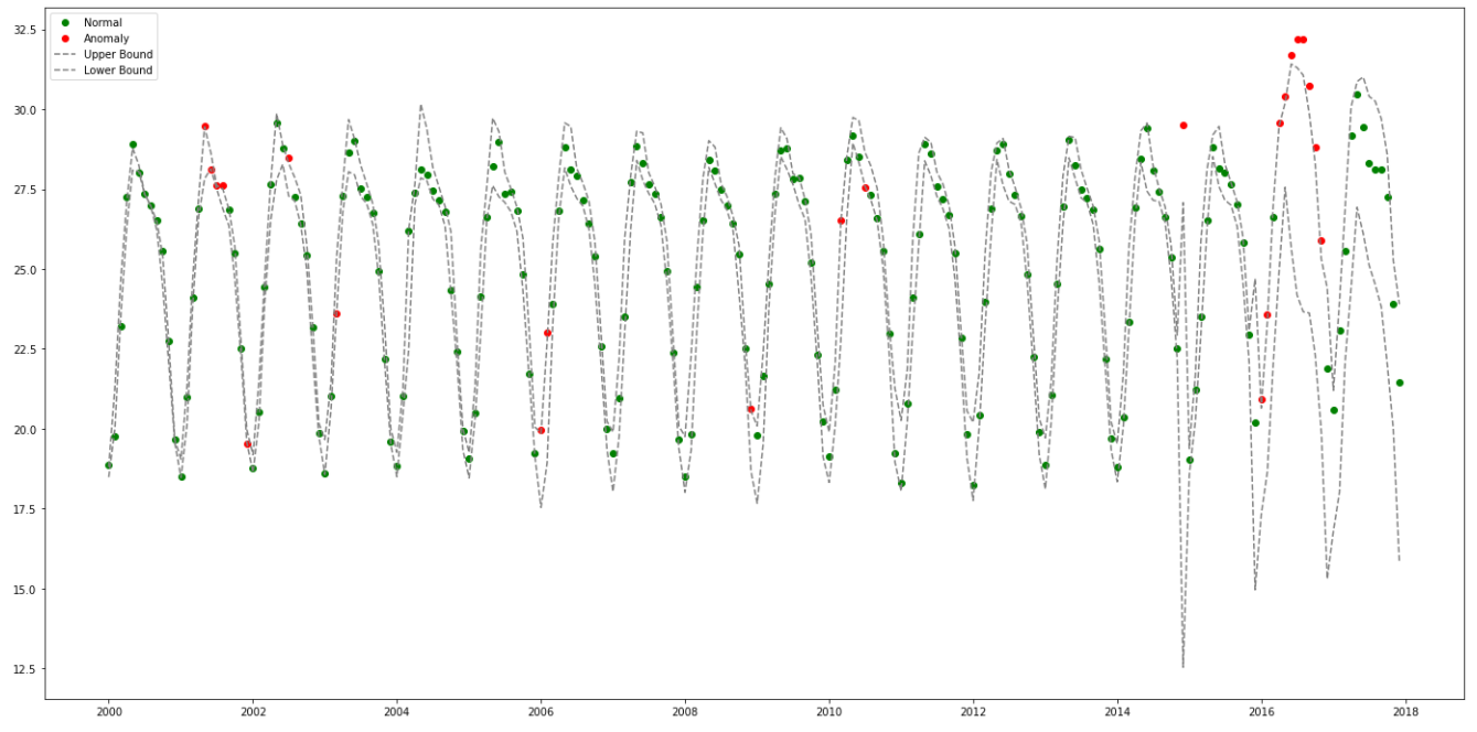
예상대로 2016에 많은 이상점들이 발견되었으나, 그 전에도 Upper/Lower Band를 살짝 넘어가는 이상 패턴들은 있었음을 알 수 있다.
'AI 빅데이터 > 후려치는 데이터분석과 AI 알고리즘' 카테고리의 다른 글
| [데이터보안] LDP ( Local Differential Privacy) (0) | 2023.01.20 |
|---|---|
| [자연어분석] Seq2Seq에 Attention 활용하기 (0) | 2021.11.30 |
| [데이터분석] Feature Engineering 7가지 팁 (0) | 2021.01.11 |
| [데이터분석] 비전을 이용한 식물 분류 (0) | 2020.11.08 |
| [데이터분석] Anomaly Detection을 위한 데이터 탐색 (0) | 2020.11.01 |


댓글